December 2022: Testing Precision in the Integration System

Table of Contents

TL;DR

If you are not interested in details:

• the precision 'as-is' exceeds specifications
• the statistical uncertainty has been improved to a level that allows investigating systematic effects

Introduction

So far, the productive bunch-2-bucket system only provided a precision about 1 ns. This is not due to imperfections of the setup, the White Rabbit network or the low-level RF system. However, the two main reasons for the 1 ns limit are the following,

• the timestamping the h=1 DDS signal is done only with 1 ns granularity and
• only one single timestamp of a single positive zero-crossing of the h=1 signal is used.

As the granularity can not be changed easily, the idea is to enhance the precision by using not only a single timestamp of the positive zero-crossing of the h=1 signal. Instead, multiple samples of consecutive zero-crossing are timestamped. Then, sub-ns precision is obtained by 'fitting' the theoretical h=1 signal - that has a known, fixed frequency - to the measured samples (details can be found here).

During fall 2022, the bunch-2-bucket test setup in the integration system has extended by two DDS systems of the low-level RF system. This allowed - for the first time - test measurements with conditions closer to reality. The result is reported here.

Setup

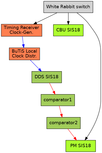Figure: Clock distribution. Shown are components propagation of rf-signals. Components of the bunch-2-bucket system are shown in light green. Components generating the reference clocks required by the DDS are shown in coral. Components involved for generating and processing the h=1 signal are shown in darker green. The arrows indicate clock propagation for White Rabbit (black), low-level RF (blue) and h=1 signal (red).

The figure above depicts clock generation and propagation. This setup is simplified compared to the real-world scenario as it does not involve the BuTiS system. Instead, 100 kHz and 25 MHz reference input clocks for the 'BuTiS Local Clock Distribution' are generated by a standard White Rabbit timing receiver. As in the production system, the DDS reference clocks are generated by the 'Local Clock Distribution' box. The DDS generated h=1 sine signals is converted to a rectangular clock signal using an internal comparator1 in the DDS; further signal conditioning is done via a second comparator2. The phase measurement is done via a White Rabbit timing receiver PM ('PM SIS18'). A central unit CBU ('CBU SIS18') communicates with the 'PM SIS18' via the White Rabbit network.

Procedure

When a fast extraction from SIS18 shall be performed, the CBU triggers a phase measurement at the PM. When the measurement is done, the PM sends the result to the White Rabbit network (the CBU then calculates the time of the kick and triggers the kicker - but this is not of relevance here). Important for this report is a second phase measurement done by the PM at the and of the extraction flat top for diagnostic purposes. Thus we have two phase measurements.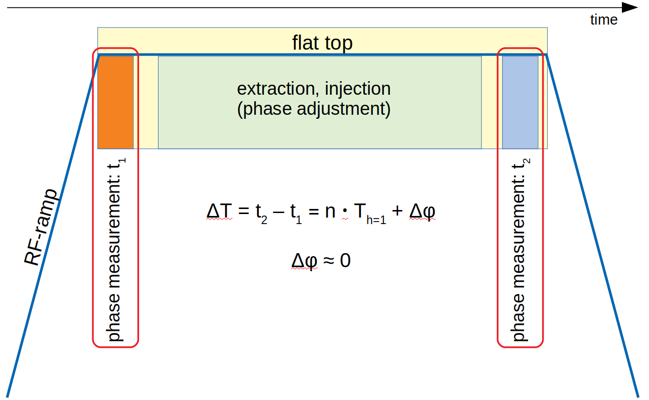

Figure: Simplified procedure of the bunch-2-bucket system. Shown are the ramp of the DDS h=1 signal (blue) and the time of first (orange) and second (blue) phase measurements.

• phase₁ (timestamp t₁ positive zero-crossing of h=1 signal)
• phase₂ (timestamp t₂ positive zero-crossing of h=1 signal)

One obtains a difference D_{t, meas} between two timestamps,

• D_{t, meas} = t₂ - t₁ .

As the DDS frequency is constant on flat-top, all time differences between two rising zero-crossing of the h=1 signal can be described in the form

• D_{t, dds} = n * T_h1 .

Under ideal conditions

• D_{t, meas} = D_{t, dds} .

Thus, one can use the system to measure a quantity

• D_phase = D_{t, meas} - D_{t, dds}

for a given number n of rf-periods. Any imperfections of the system will show up as non-zero value

• D_phase ! = 0 .

The bunch-2-bucket system has been extended to higher precision by implementing the new analysis procedure in the FPGA in real-time. The result of that analysis yields D_phase together with an estimated uncertainty. The PM unit publishes the data in real-time via the CMD_B2B_DIAGEXT message to the White Rabbit network. By this, the data can easily be obtained, archived and analysed.

Measurements

Resolving Power

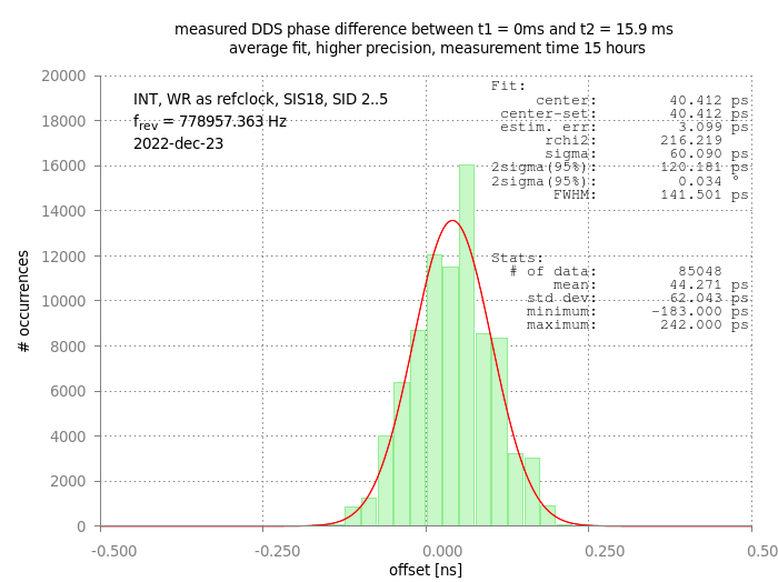
The first measurements (see above) have been obtained by using 20 samples per single phase measurements. Increasing the precision - and resolving power - can be achieved by using more samples. As a first step, the number of samples has been increased up to 200.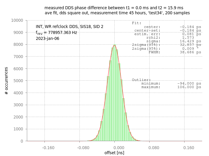

Figure: Measured phase difference for 200 samples (per single phase measurement). A Gaussian fit is done to the histogram.

In the figure above, 65264 measured phase differences are plotted as a histogram. A Gaussian fit yields a FWHM of 39 ps only. It is interesting to note, that such a small width is obtained even with an overall measuring time of has been 45 hours. This illustrates that the system itself is robust and works extremely stable. Please note the maximum/minimum deviation of the outliers is just ~100 ps.

Line Shape

Width vs Jitter

In the following the resolving power was increased by using more samples per single phase measurement. This was done up to 200 samples to get a better understanding of the overall system. Remark: For real operation such a high number of samples is probably not useful as this increases not only the measurement time (here: 200 * 1.283 us = 256 us) but also increases the time required for data analysis in the FPGA.

As an analytical model of the line shape does not exist, numerical simulations were performed that can be compared to measured data. To get a first estimate on the relative 'jitter' between White Rabbit and DDS clock signals, simulations have been performed for different values of the jitter as input data. Each simulation typically included 100000 'extractions' and assumed a normal distribution (Gaussian shape) for the 'jitter' distribution.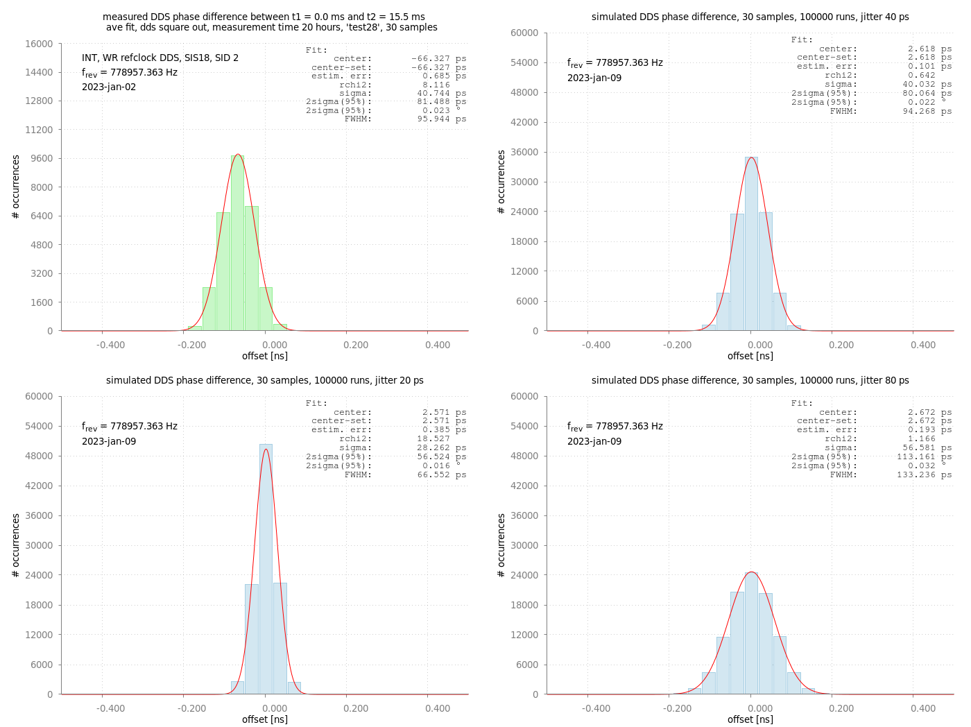

Figure: Green: Measured distribution of phase differences with 30 samples per single measurement. Blue: Simulated distribution of phase differences for three different input values for 'jitter'.

The figure above compares the measured data to simulated data for for jitter values of 20 ps, 40 ps and 80 ps. The shape obtained for a jitter value of 40 ps fits the experimental data best.

Width vs Number of Samples

The line-width of measured data not only depends on the jitter between the DDS and White Rabbit clocks but also on the number of samples used for the phase measurement. This was investigated by measured and simulated data, by varying the number of samples from 20..200. The result is plotted in the figure below.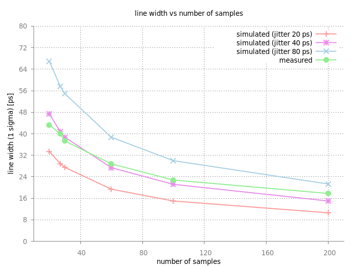

Figure: Standard Deviation (fit: 1 sigma) as a function of number of samples. Measurement: green, solid. Simulation for different assumed jitter values: red (20 ps), blue (40 ps), yellow (80 ps), dashed. The statistical uncertainties are smaller than the plotted symbols.

As can be seen, the width of the distribution decreases with increasing number of samples. Both, measurement and simulated data show the same behavior. When comparing the measured data to simulations performed for different jitter values, the best match is obtained for jitter value of 40 ps. As a tentative result one can assume the concerned clocks have a relative 'jitter' in the order of 40 ps.

However, the simulation slightly overestimates (underestimate) the width of the distribution for low (high) number of samples. This can not be explained by the statistical uncertainty; a systematic effect not included in the simulation might play a role.

Micro Structure

The nature of the measurement leads to a micro structure of the acquired data. The idea of the measurement is similar to the one described here. While the 'sub-ns-fit' just uses the two extremes, the measurements described here used an 'average-fit'. A single measurement uses several samples (timestamps) of h=1 rising edges. Each rising edge delivers a sample (timestamp) with 1 ns granularity. If multiple samples are used:

• 1 sample: the average is full nanoseconds only
• 2 samples: the average has distinct values of 1/2 nanoseconds
• ...
• 10 samples: the average has distinct values of 1/10 of nanoseconds

As a result, all phase differences have a 'comb-like' micro structure that shows up, if histograms of many measurements are plotted with very small bin-width.

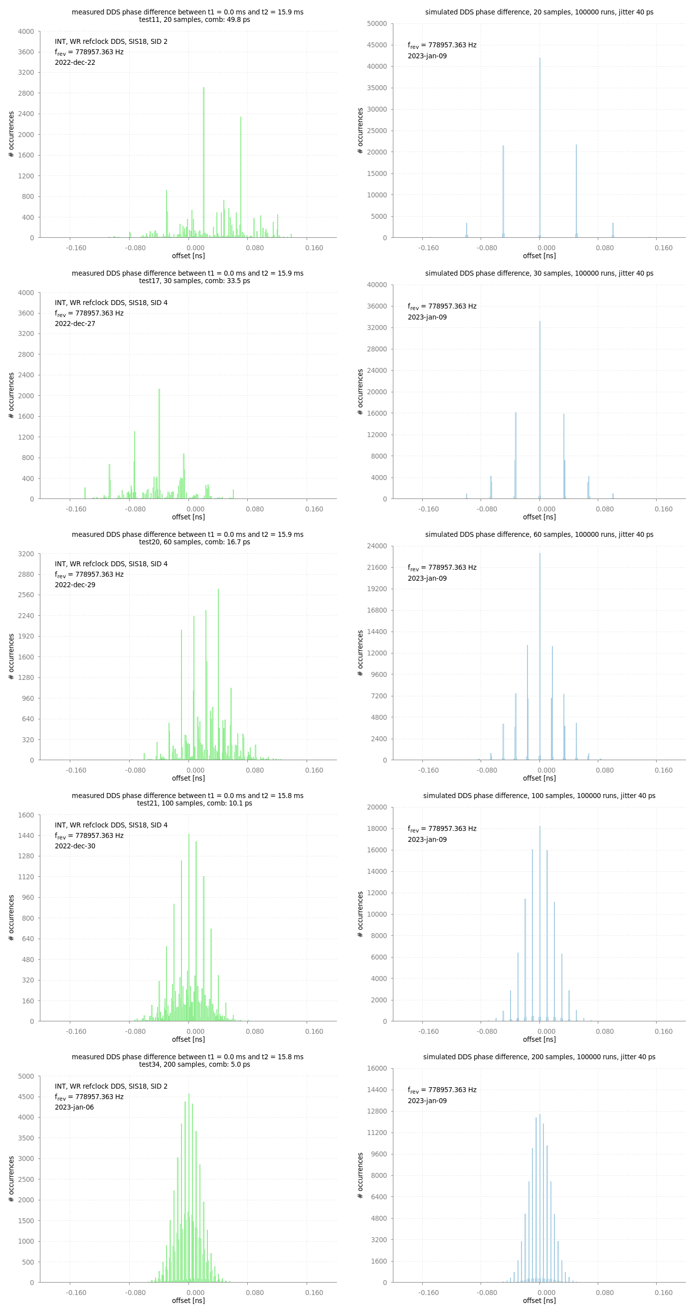Figure: Comb-like micro structure. Each histogram shows number of occurrences as a function of phase difference. Shown are measured (left) and simulated (right) data. The number of samples used for phase measurement is increased from top to bottom.

The figure above shows a comb-like micro structure for measured and simulated data for a different number of samples. It is interesting to note, that the measured data has some particular noise that can not be reproduced by the simulation.

Observation of Systematic Effects

The booster pattern SIS18_FAST_HHD_BOOSTER_20220615 consists of four booster cycles. As all booster cycles have the same energy energy at flattop, the measured phase difference of all four booster cycles should have an identical value (preferably 0 ps). However this is not the case, as can be seen in the figure below.

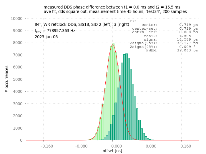Figure: Measured phase differences for two different booster cycles. A Gaussian fit is done to the histogram of SID 2.

As can be seen, the mean value for the two booster cycles is clearly different. As the data for all four booster cycles is measured 'simultaneously' during the same time span (here: 45 hours) long term drifts can be excluded.

Long-Term Drifts

The figure below shows a long term measurement of about 6 days has been performed to check for long term drifts of the four booster cycles with SID 2..5.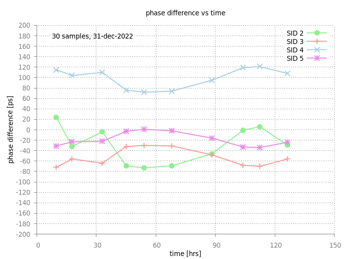

Figure: Measured phase difference vs time of the four different booster cycles. No error bars are shown as the statistical uncertainties of the phase differences are smaller than the symbols. The measurement has been started on 31 December around 0943 UTC.

For this measurement, the number of samples has been reduced to 30. Besides the booster pattern, another pattern in SIS18 (to ESR) was operational about every 20 seconds. To check for possible correlation, the other SIS18 pattern to ESR was disabled every 2nd measurement. However, no clear correlation is observed. Slow drifts over days are observed. However, it is evident, that the measured phase differences are non-zero and distinct for all four booster cycles.

Short-Term Drifts 1

As the long-term measurement did not give any clue on the non-zero phase differences, short-term drifts were investigated.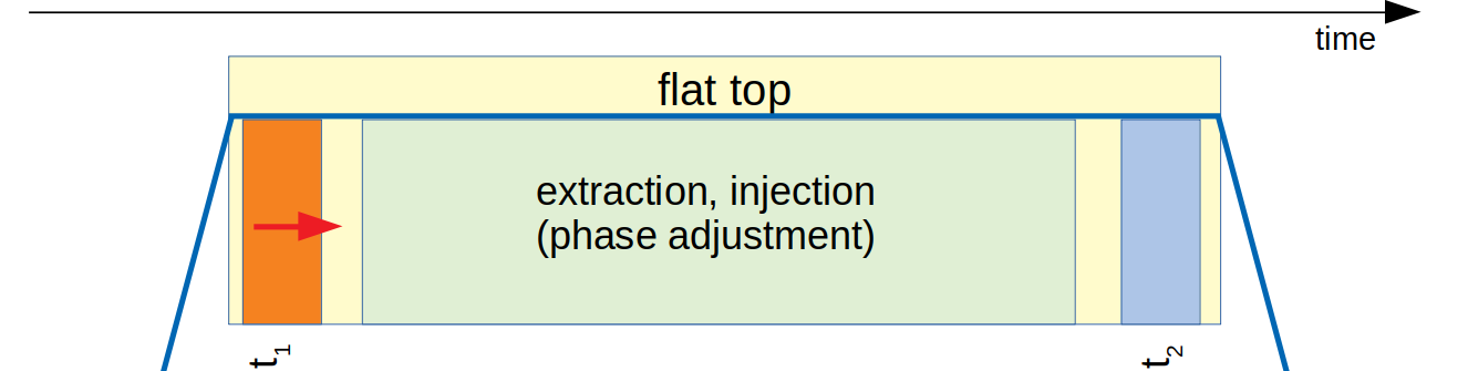

Figure: Modified Bunch-2-Bucket procedure: The window for the first phase measurement window at the beginning of the flat top is delayed.

Here, the first phase measurement at the beginning of the flat top was slightly delayed. The result is shown in the figure below.

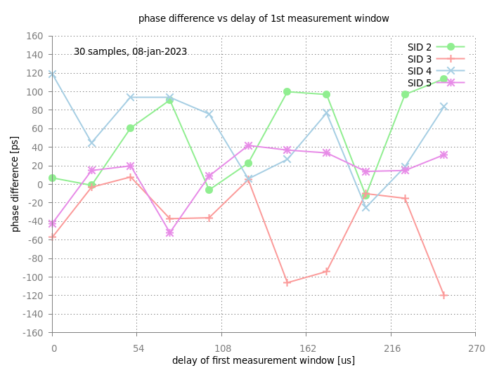Figure: Phase difference versus delay of the 1st measurement window at the beginning of the flat top. Error bars are not shown, as the statistical uncertainty are smaller than the symbols.

The result is not very conclusive. If the measurement window is delayed, the measured phase differences shift significantly. This is not expected. Although the complete measurement took about 16 hours, long term drifts can not explain the magnitude of the observed shifts. Some of the data points have been measured on Monday morning (9 January) and one could speculate, if unstable conditions might have played a role. At that time, it was not possible to continue the measurements due to ongoing maintenance work in the facility. These measurements shall be repeated in cleaner conditions.

Short-Term Drifts 2

Two phase measurements are done on flat-top. The first (second) measurement is done in a 'measurement windows' at the beginning (end) of the flat-top. The phase-difference is then calculated from these two measurements. To check for effects such as frequency drifts at the end or beginning of the flat top, the first or last phase measurement have been shifted systematically towards the center of the flat-top. In total six series of measurements have been done.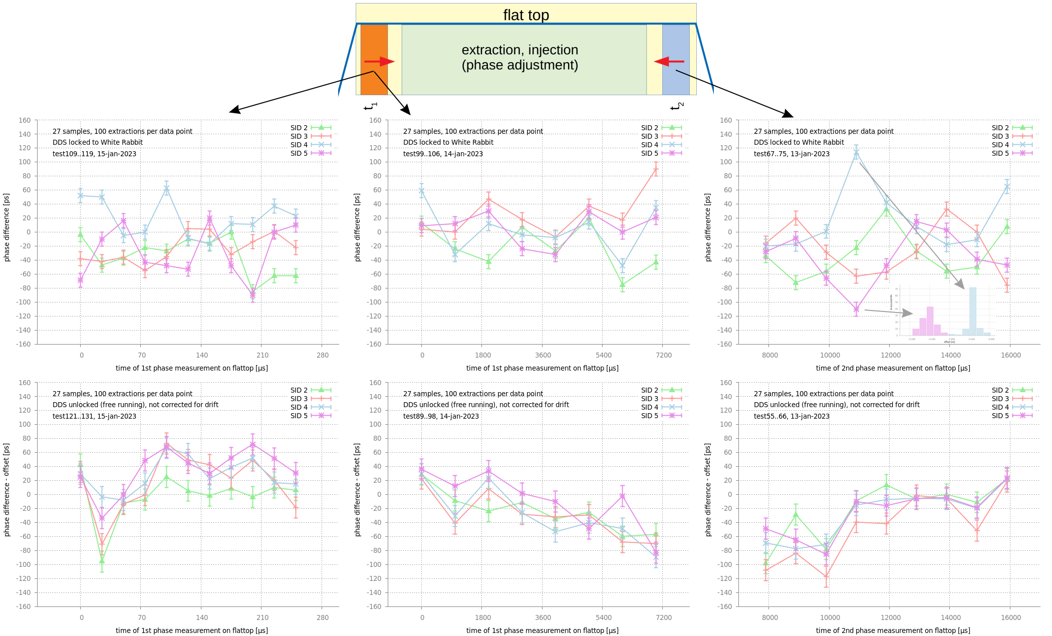

Figure: Phase differences as a function of position of measurement windows for the four different booster cycles with SID 2..5. Left: 1st window is shifted in steps of 25us. Middle: 1st window is shifted in steps of 1000us. Right: 2nd window is shifted in steps of 1000us. Top: DDS locked to White Rabbit. Bottom: DDS not locked (free-running on internal clock). Each data point is an average of ~100 measured phase differences. The inset in the top-right figure depicts histograms at t₂ ~ 10900 us for SID 4 and 5. Details see text.

The figure above shows the result of three different measurements (top). As it was assumed, that phase value of the h=1 signal at the beginning of the flat top plays a role, these three measurements have been repeated under the same conditions (bottom) with free-running DDS systems (using the internal clock only). This was done, because then the h=1 (free-running) DDS signal at the beginning of the flat-top does not have a defined but a random value with each iteration. As the frequency of the free-running DDS system is different, all values are corrected by an offset.

The curves with free-running DDS show a systematic slope which is due to a slow frequency drift. The total measurement time for each of the six plots shown is about 1 - 2 hours. During this time, the observed frequency of the h=1 signal typically drifts by a couple of milli-Hertz. The plotted data is not corrected for this drift and the slope should be neglected.

Although all figures look very noisy, it is important that the differences of the values are statistically significant. The plotted values are the center value of a Gaussian function fitted to histograms. The inset in the top-right figure shows an example of the 'raw data', namely the histograms for SID 4 and 5 at t₂ = 10900 us. As can be seen, the two histograms for the two different SIDs are two clearly separated peaks. Another important thing: Those peaks do not shift even when adding data of many hours.

Two series (top-left, top-middle) have been done where the first measurement window has been shifted towards the center of the flat-top. Bottom-left and bottom-middle: The difference between the four booster cycles seems less pronounced with free-running DDS. But it is interesting to note, that the measurement values for SID 2 (green) are systematically lower for SID 3..5. The differences between SID 2..5 do not disappear, when the measurement window is shifted.

Another series (top-right) has been done by shifting the 2nd measurement window towards the center of the flat-top. Also here, the scatter does not disappear.

Simulations on Short-Term Drifts

Phase Difference versus Number of Samples

The reason for the short-term drifts is unknown. As a speculation, the shift of the measurement window might have a small effect on the number of samples that are effectively used for the phas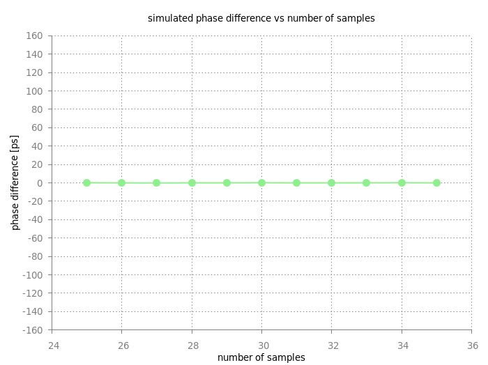e measurement.

Figure: Simulated phase difference for varying number of samples.

To exclude this possibility, numerical simulation were done with varying number of samples. As shown in the figure above, the simulation can not explain shifts that are of the same magnitude as observed by the measurement.

Phase Difference versus h=1 Phase

Another speculation: Does the phase of the h=1 DDS signal with respect to the start of the measurement windows does influence the value of first measured phase value?

Shifting by an Integer Number of Nanoseconds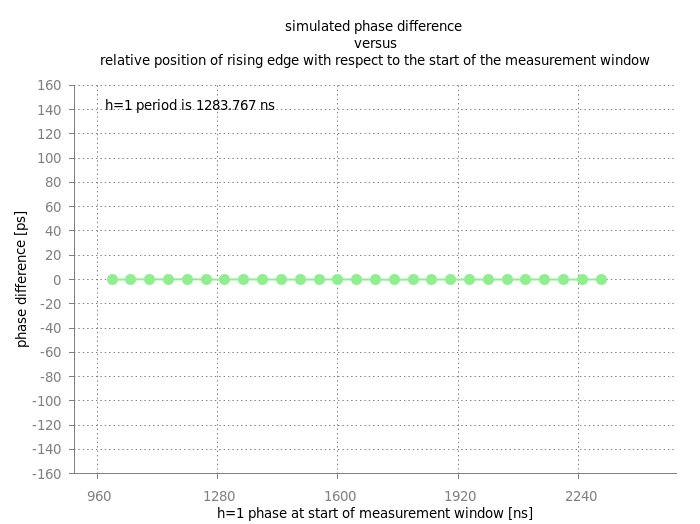

Figure: Simulated phase difference. Here, the rf-phase at the start of the measurement window has been changed in units of several nanoseconds.

To exclude this possibility, numerical simulation have been performed where start of the measurement window was shifted by an integer number of Nanoseconds. As shown in the figure above, the simulation can not explain the shifts observed in the experiment.

Shifting by Sub-Nanoseconds

In timestamps in full nanoseconds are available for the fit algorithm (click). The fit algorithm determines the fractional part of the measured phase only. Thus, shifting the timestamps by full nanoseconds does not change the fractional part. However, small shifts of sub-nanosecond scale might cause one or more h=1 signals to be shifted into neighboring nanosecond bins (basically, this leads to the 'comb-like' micro-structure in the histograms).

It was observed, that each of the four booster cycles has a fixed h=1 phase at the beginning of the flat top. If this phase is defined better than one nanosecond, sub-nanoseconds shifts must be considered.

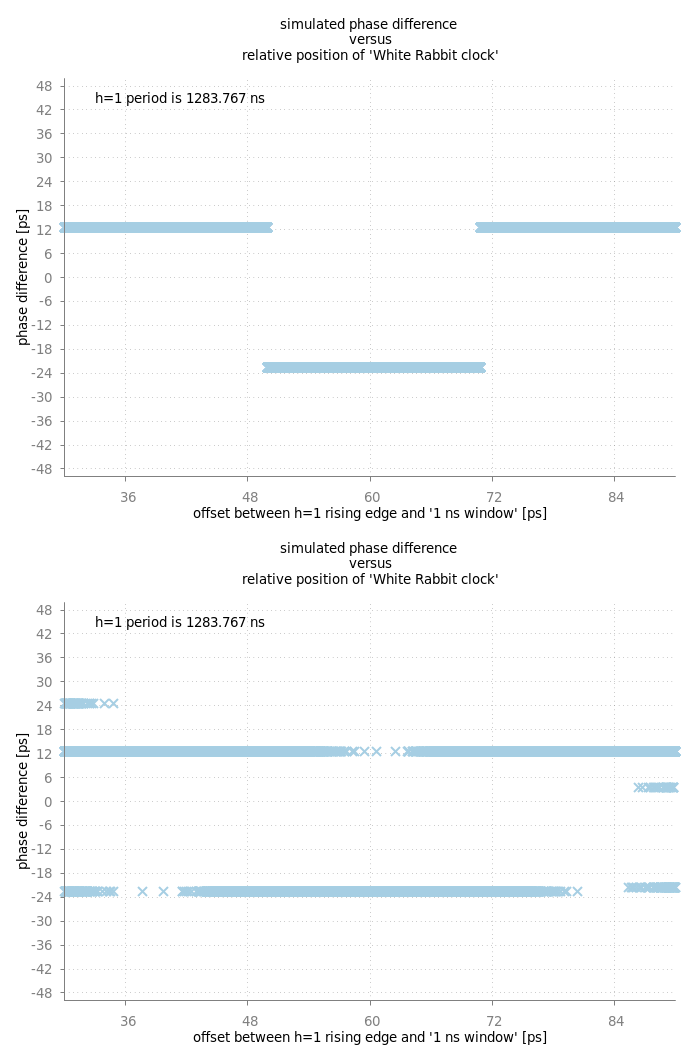Figure: Simulated phase difference. Here, the rf-phase at the start of the measurement window has been changed in sub-nanoseconds. Top: no jitter. Bottom: jitter 3ps standard deviation.

The figure above shows a simulated example, how the phase difference is shifted, when the rising edge of the h=1 signal is slightly changed relative to a full nanosecond. The simulation was done with parameters resembling the true setup, but without any jitter-noise (top). As explained here, if the acquired timestamp of a h=1 zero-crossing shifts to a neighboring nanosecond bin. The pattern is irregular and sometimes it happens, that multiple rising edges shift to neighboring bins. The simulation yielded a window of about +/- 35 ps for a single phase measurement. Thus, phase differences may vary in a windows of about +/- 70 ps. However, this effect washes out quickly, if noise in the low two-digit range is added to the the simulation (bottom).

Again, this does not explain the inconsistencies of the measured phase differences up to +/- 120 ps.

Discussion on Non-Zero phase differences

Non-zero phase differences have been observed in the experiment:

• all four booster cycles show different values of phase differences
• even when measuring over many hours, the phase differences stay stable
• significant shifts outside statistical errors can be triggered when changing the position of the first measurement windows with respect to the start of the flat top
• 'clock jitter' can not explain the non-zero phase differences
  • increasing the clock jitter in the simulation does not change the phase difference
  • the 'jitter' of the setup is estimated to be in the order of 40 ps; this is significantly lower the the observed shifts

It was confirmed with colleagues from system planning, that rounding of the rf-ramps at the beginning or end of flat top might play a role. According to the model, the frequency shall be constant at the set-value on the flat top.

If the function generator delivers a constant value for the DDS, it can be excluded that this value is wrong. The DDS uses a 200 MHz input clock and has a resolution of 32 bit. Thus, the DDS can only produce distinct frequencies with a step size of

• ~46.6 mHz

Thus, if the set-value of the DDS would be wrong by 1 bit, a frequency shift of ~46 mHz would be observed. However, the largest deviation of the measured phase-difference from the '0-value' is in the order of 100ps, which corresponds to

• ~4.9 mHz

only.

Would a periodic oscillation, drift of the White Rabbit clock versus the generated h=1 RF signal explain non-zero phase differences?

• The length of the measurement window for 30 samples at this frequency is about 40 us. A periodic oscillation much shorter than 40 us would cancel out due to the averaging of many samples.
• The length of the complete booster pattern is less than 2 seconds. An oscillation in the order of a couple of seconds might possibly lead to a shift of the phase difference. However, this would affect all booster cycles in the same way.
• Even if an oscillation has a period somewhere in between 40 us and a few seconds, it is hard to believe that this could explain that
  • the phase-difference for each SID remains constant over many hours AND
  • the phase-difference for each of the four booster cycles has a different value.

The function generator for the rf-ramp runs continuously for the last three booster cycles. Thus, the phase of the h=1 signal at the beginning of the flat top is almost fixed for a specific booster cycle. However - using an oscilloscope - it has been verified that the phase of the h=1 signal has a different value at the beginning of the flattop (the oscilloscope is triggered at flattop start) for each of the booster cycles. According to the simulation, this does not play any role for the result of the measurement if the reference clocks of the low-level rf-system and White Rabbit are phase locked to each other (this is the case!): Even assuming a large jitter between the clocks, it is not possible to reproduce non-zero phase differences.

Non-zero phase differences up to 100 ps can not be reproduced by the numerical simulations. However, the simulation always assumed that the mean frequency of the h=1 signal is constant. Minute shifts or variations of the involved frequencies are not considered yet.

On the one hand, the observed magnitude of the non-zero phase differences is fairly small. Considering the requirements of the bunch-2-bucket system, this effect could be neglected. On the other hand, the source of the effect is unknown and it might become larger/relevant in different conditions.

Conclusion on Non-Zero phase differences

Phase differences of DDS h=1 signals can be measured with a statistical precision in the low two-digit picoseconds range.

The measured phase-differences show deviations of statistical significance from the zero value. However, these deviations are typically smaller than 100 picoseconds.

Surprisingly, the measured phase-differences are not identical for the four booster cycles. The discrepancies don't disappear even when measurement over many hours.

At present it is not possible to decide, if the measured non-zero phase differences are real or an artifact of the overall system.

Ideas:

• repeat measurement using a special pattern with constant (!) frequency of the h=1 signal (no ramping)
• using BuTiS as reference clock for the low-level rf-system

Final Conclusion

Phase differences can be measured with sub-ns precision. Systematic effects play a role when measuring with high resolving power.

A precision of about 100 picoseconds can be achieved.

Future Operation

The measurements presented here were performed in clean conditions. For operation in the real facility, the precision might be deteriorated. Effects including the following must be investigated

• The reference clocks of the low-level are not generated by the White Rabbit hardware but using the BuTiS system. Potential differences between the BuTis and White Rabbit clocks need to be considered. On the one hand, the jitter of the DDS signal will decrease (!), but relative drifts might start to play a role.
• As can be seen here, the number of White Rabbit switch layers will increase. It needs to be tested, in how far this affects the uncertainty of measured phase differences.
• The setup for the measurements presented here is installed in a single rack; this might be different in the production environment.

Bonus: Free-Running DDS

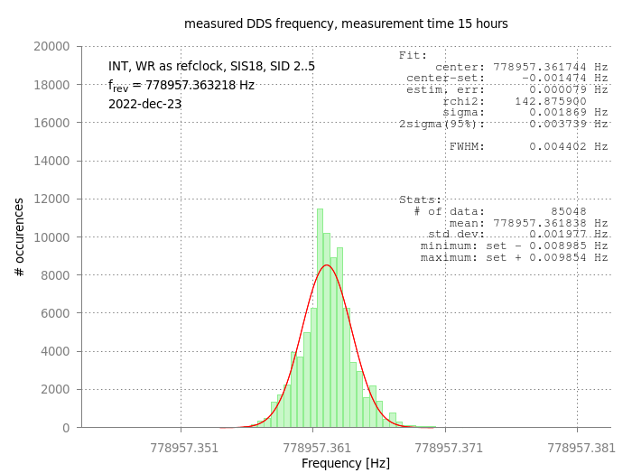
As a cross-check, the measurements of phase and frequency differences described above hav been repeated. However, the reference clocks to the 'Local Clock Distribution' box have been disconnected. Thus, the h=1 DDS were operated on the internal clock only, 'free running'.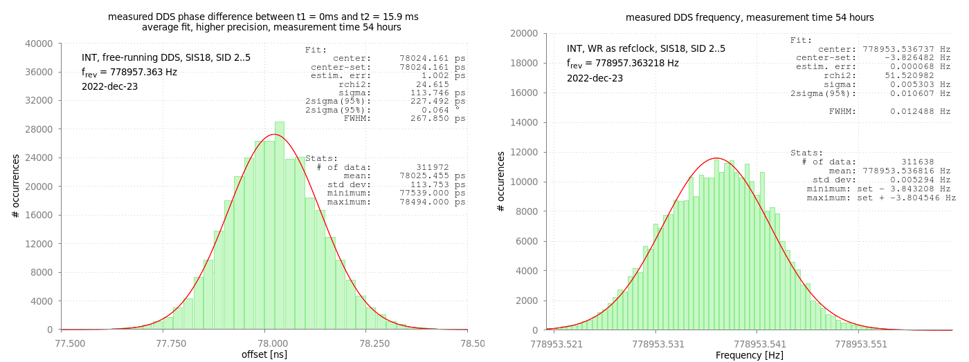

Figure: Left: Measured DDS phase difference between two positive zero-crossings of the h=1 signal. Right: Measured DDS frequency. The DDS operated 'free running', using the internal clock only.

As expected, a drastic change is observed when the DDS is switched to 'free running' mode. As shown in the figure above, rhe frequency of the output signal is reduced by about 3.8 Hz and a huge jump of the measured DDS phase difference is observed. As can be seen, the phase difference is off by about 78 ns and frequency shifted by about 3.8 Hz. Moreover, the distributions is slightly broader which is most likely caused be frequency drifts of the internal clock.

-- DietrichBeck - 10 Jan 2023