Sub-Nanoseconds Phase Fit

Method

The sub-ns phase fit algorithm can increase the preceision of time stamped data points from a periodic signal to values below the sampling resolution of 1 ns. Application: measure zero-crossings of a ring-RF-signal with sub-ns precision using a standard FAIR Timing Receiver.

• The algorithm is evaluating the "phase difference", the difference of the measured time of a zero crossing to the expected RF-phase value based on the known RF-period. This picture illustrates how the phase difference is calculated. The time measurements have a sampline resolution of 1 ns.
  

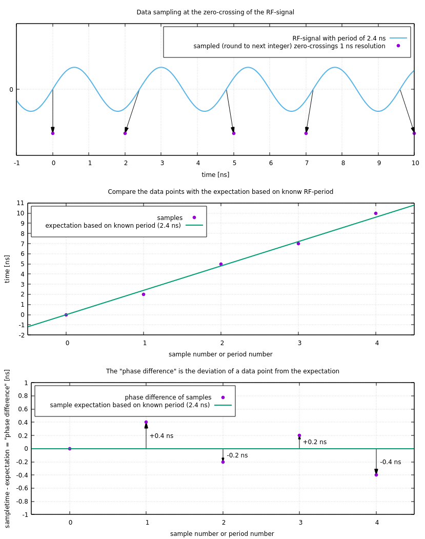
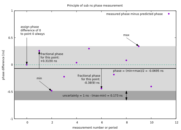
• How the sub-ns phase fit works (in principle): Find min and max of the phase difference. The best estimate for the phase offset is (max+min)/2. The uncertainty is 1ns-(max-min).:
  

Performance with Jitter

Performance of sub-ns phase fit algorithm for simulated data. The columns show a different jitter strength (+- 100 ps means that a randum number in the interval [-100 ps, 100 ps] is added to each value before discretisation to 1 ns resolution. The first row shows how the result of the algorithm deviates from the simulated input value. The second row shows the same, but fractional part of the result was truncated to 3 bits (125 ps) resolution. The quality of the result depends on the fractionl part of the period number of the RF-frequency. For periods that are integer multiples of 1 ns, the algorithm cannot determine a sub-ns phase value.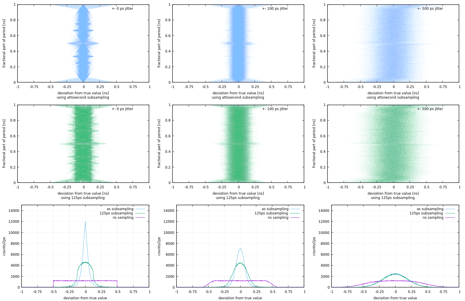

The performance of the algorithm was measured in the INT-iinstance of the B2B system. A series of phase values, with 125ps resolution was recorded by snooping for the respective event on one of the nodes (scuxl0288): saft-ctl tr0 snoop 0x13a0802000000000 0xfffffff000000000 0 > b2b_phases.dat

The phase value is stored in the parameter field of each event. For each phase value in the series of measurements, the time difference to the previous phase value dt was calculated. The number of RF-periods N was calculated based on the known RF-period T. The difference dp-N*T was sorted into a histogram. The procedure was done for the 125ps resolution, and for 1n resolution (by truncating the last 3 bits). The difference peak using the 125ps resolution values is 3.8 times narrower (FWHM) than the one from the 1ns resolution values. The resolution of a single phase value measurement can be calculated by dividing the width of the difference peak by sqrt(2) (indicated by the yellow Gaussian function in the picture below). The FWHM of the single measurement is 0.18 ns. The orange line (trinagular shape) shows the expected shape of a uniform distribution with 1 ns width, folded with itself (as is expected when calculating the difference).

Performance of Algorithm (Monte-Carlo)

The accuracy of the algorithm depends on the fractional part of RF-period (in ns). The worst cases are:

• fractional part is close to 1 ns / 1, really bad
• fractional part is close to 1 ns / 2, bad
• fractional part is close to 1 ns / 3, not so good
• ...

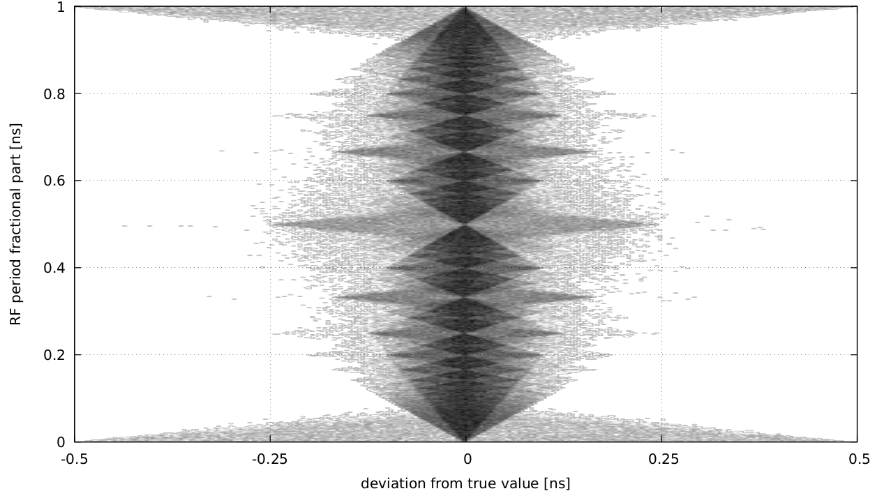Figure: Deviation from true value (x-axis) as a function of the fractional part (1 ns) of the rf-period.

The figure above was obtained by Monte-Carlo simulations, where the initial RF-phase, RF-period, and jitter was included. As can be seen, the algorithm yields bad performance if the fractional parts are close to 1 ns divided by an integer number; the worst scenario is obtained if the rf-period is close to one full nanosecond.

Performance of Algorithm (Model)

The relationship between accuracy and fractional part of the RF-period and -phase is a systematic effect. As the size of this effect must be known to understand systematic deviations observed during on-line operation of the accelerator, a Monte-Carlo method is not suitable. Hence, a simple model was developed that describes the maximum deviation of a single measured RF-phase from its true value. The only free parameters of this model are the RF-period and the number of samples. In order to estimate its correctness, the output of the model is compared to numerical simulations, where the maximum deviation from the true value is simulated. The figures compare model and simulation for a different number of samples. In order to demonstrate the pure systematic effect, the data shown here have been obtained without considering any jitter

Description of figures

• y-axis: deviation of the rf-phase determined via the sub-ns fit from the true value
• x-axis: fractional part of the RF-period
• blue: model (left y-axis)
• orange: simulation (left y-axis)
• yellow: residuals, simulation - model (right y-axis)

From top to bottom

• 30 samples
• 10 samples
• 3 sample

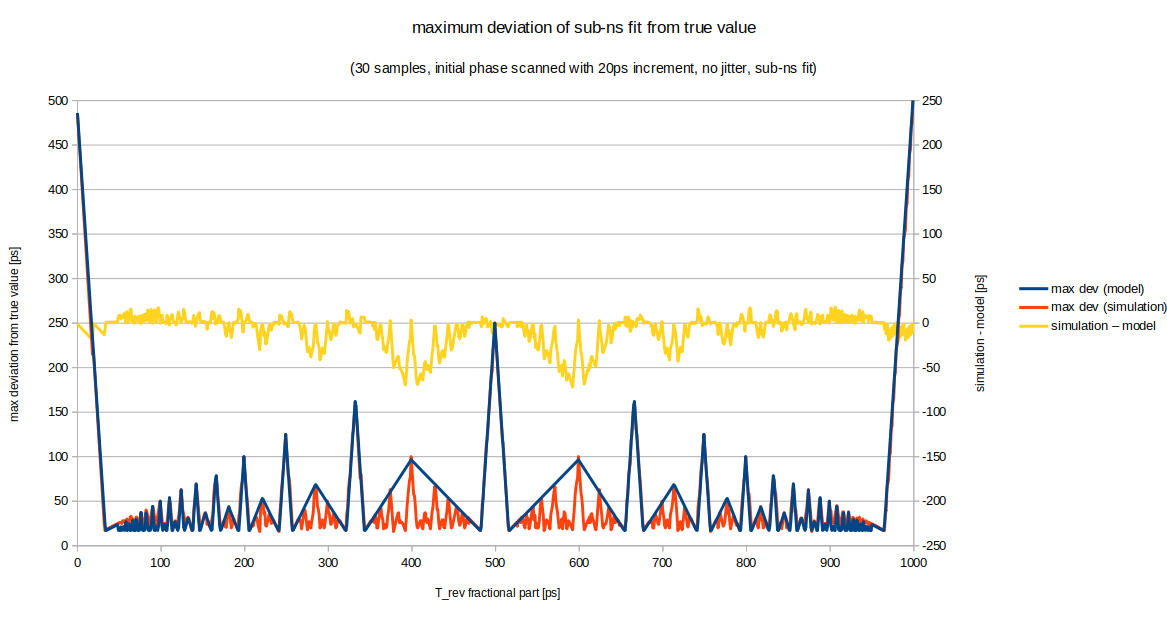
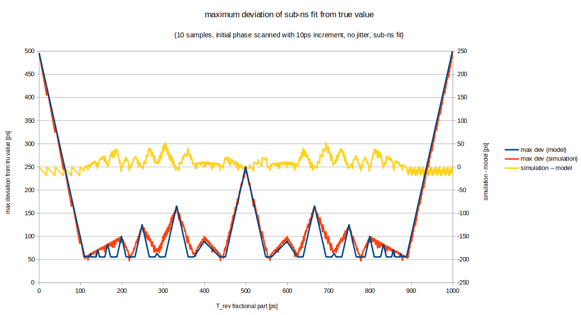
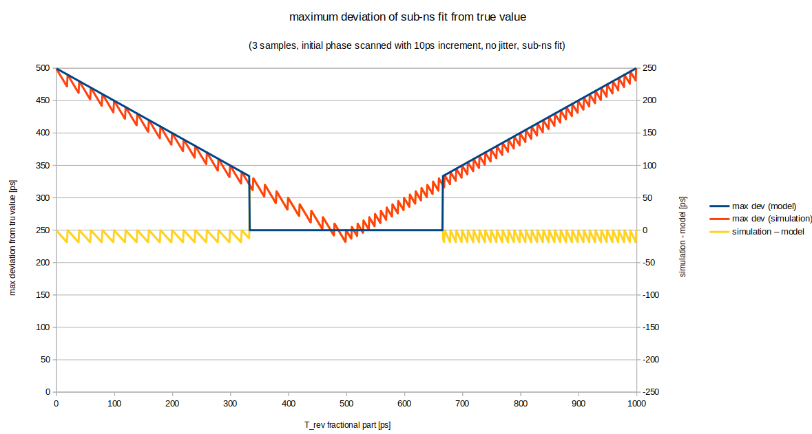The trend of the original Monte-Carlo simulations is reproduced.

All three figures demonstrate a good match of the model to the simulated data; in general the agreement between model and simulation is better than 50 ps.

It can be seen, that the average deviation of the sub-ns fit result from the true value is reduced by increasing the number of samples.

The model is coded into a simple routine written in c-code (bel_projects, branch b2b_dietrich_2023-apr-28, commit 9bfb00ea7), it's execution only requires negligible CPU time. It is planned to include the result of the model into the on-line analysis of the b2b system. This will allow a better understanding in case the monitoring/measurements of the on-line analysis yield a deviation outside the statistical uncertainty.

-- MichaelReese - 11 Apr 2022, DietrichBeck - 15 Sep 2023